Reaction-Diffusion by the Gray-Scott Model: Pearson's Parametrization
Introduction
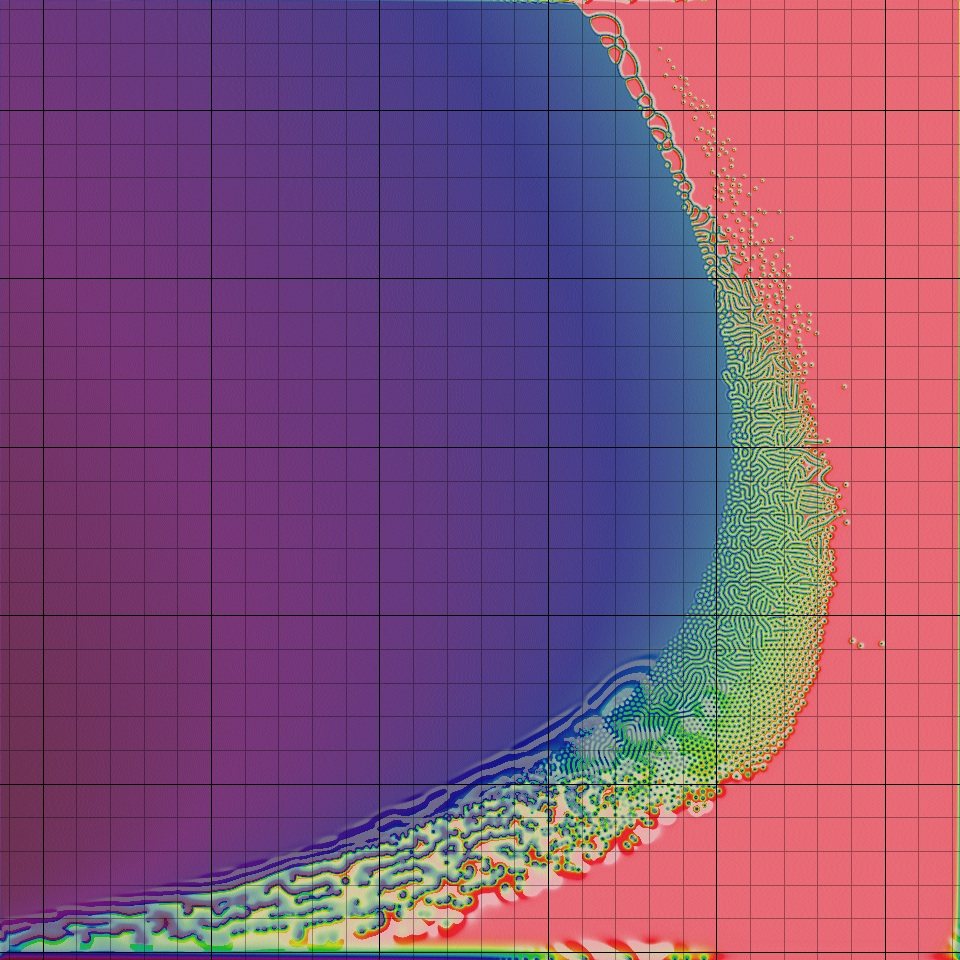
Instructions: A click anywhere in the crescent-shaped complex region will take you to a page with images, a movie and a specific description. Each grid square leads to a different page.
You may prefer to browse the different patterns by starting with my extension of Pearson's classification of the types of emergent behaviours. I also have special pages for the U-skate world and certain other very exotic patterns, and a Gray-Scott nomenclature glossary.
This web page serves several purposes:
|

This work led to new discoveries and scientific investigation described below.
What Is It?
All of the images and animations were created by a computer calculation using the formula (two equations) shown below. In Roy Williams' words, it is a "relatively simple parabolic partial differential equation". Details are below; the essence of it is that it simulates the interaction of two chemicals that diffuse, react, and are replenished at specific rates given by some numerical quantities. By varying these numerical quantities we obtain many different patterns and types of behavior.
The patterns created by this equation, and other very similar equations, seem to closely resemble many patterns seen in living things. Such connections have been suggested by:
- Turing, 1952 [1] (dappling; embryo gastrulation; multiple spots in a 1-D system)
- Bard and Lauder, 1974 (leaves, hair follicles)
- Bard, 1981 [2] (spots on deer and giraffe)
- Murray, 1981 (butterfly wings)
- Meinhardt, 1982 [3] (stripes, veins on leaf)
- Young, 1984 (development of eye)
- Meinhardt and Klinger, 1987 (mollusc shells)
- Turk, 1991 (leopard, jaguar, zebra)
and many more in more recent years. Beginning with Lee et al. [7] and Pearson [8] the field broadened, greatly facilitated by computer simulation.
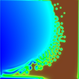
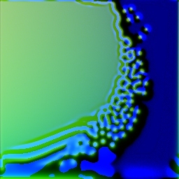
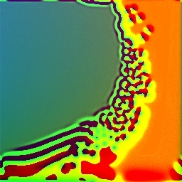
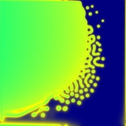
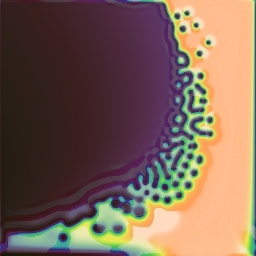
Some of the colour maps I tried
In his original 1994 exhibit3, Roy Williams presented grayscale images for many pairs of k and F, each showing a "histogram-equalised view of the U component". He suggested that the images, after modification by "a little playing with the colour map" would be "quite attractive as gift-wrapping". My images, like Williams', meet their own edges seamlessly, so they would look good if you used them as wallpaper on your computer monitor, for example.
The organic appearance and great diversity of patterns makes Gray-Scott patterns ideal for purely artistic applications, such as my own screen saver:

The Xmorphia PDE5 screen saver
You can download this screensaver here
Colouring Gray-Scott for Serious Work
Even for fairly non-artistic purposes such as a scientific publication, much attention should be given to the visual presentation of the simulation data.
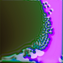
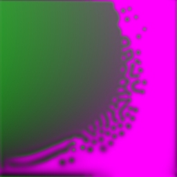
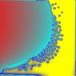
Another 4 trial colour maps
For this website, I wanted to express more than one dimension of information (specifically: u and ∂u/∂t) and I wanted the colour mapping to be the same everywhere in the system, so that any two images could be compared directly with the knowledge that identical colours always represent identical values of u and ∂u/∂t. This prevented the approach of using "histogram equalization" or anything that changes the mapping from data value to colour.
In addition to meeting those basic requirements, the colour scheme I ended up with meets all of the following objectives:
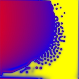
- Low u values, including the large plain area near the left, are "blue", while high u values and the area on the right are "red" — this is to match the colours used by Pearson in his paper [8] which in turn match the colour of the pH indicator bromothymol blue used in actual experiments such as [7];
- The colours make fairly full use of the entire HSV (hue-saturation-value) colour space, in an aesthetically pleasing way;
- With practice the observer can distinguish the level of u as well as the rate of change of u, and neither one obstructs the other;
- Resulting images compress well into JPG and H264 video without producing distracting artifacts or exceeding the colour gamut of those standards.

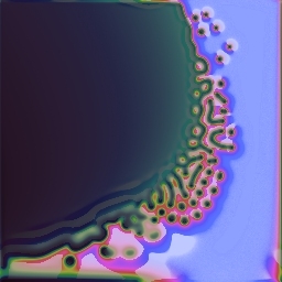
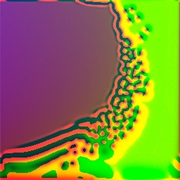
Another 4 trial colour maps
The Formula
The reaction-diffusion system described here involves two generic chemical species U and V, whose concentration at a given point in space is referred to by variables u and v. As the term implies, they react with each other, and they diffuse through the medium. Therefore the concentration of U and V at any given location changes with time and can differ from that at other locations.
There are two reactions which occur at different rates throughout the space according to the relative concentrations at each point:
U + 2V → 3V
V → P
P is an inert product. It is assumed for simplicity that the reverse reactions do not occur (this is a useful simplification when a constant supply of reagents8 prevents the attainment of equilibrium). Because V appears on both sides of the first reaction, it acts as a catalyst for its own production.
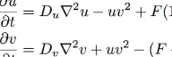
The overall behavior of the system is described by the following formula, two equations which describe three sources of increase and decrease for each of the two chemicals:

The Reaction-Diffusion System Formula
u=[U], the concentration of U, and v=[V]. For the sake of simplicity we can consider Du, Dv, F and k to be constants. In computer simulations there are also quantization constants for time and space (Δt and Δx) that are used to break ∂t and ∇2 into discrete intervals.
The first equation tells how quickly the quantity u increases. There are three terms. The first term, Du∇2u, is the diffusion term. It specifies that u will increase in proportion to the Laplacian (a sort of multidimensional second derivative giving the amount of local variation in the gradient) of U. When the quantity of U is higher in neighboring areas, u will increase. ∇2u will be negative when the surrounding regions have lower concentrations of U, and in such cases the diffusion term is negative and u decreases. If we made an equation for u with only the first term, we would have ∂u/∂t = Du∇2u, which is a diffusion-only system equivalent to the heat equation.
The second term is -uv2. This is the reaction rate. The first reaction shown above requires one U and two V; such a reaction takes place at a rate proportional to the concentration of U times the square of the concentration of V6. Also, it converts U into V: the increase in v is equal to the decrease in u (as shown by the positive uv2 in the second equation). There is no constant on the reaction terms, but the relative strength of the other terms can be adjusted through the constants Du, Dv, F and k, and the choice of the arbitrary time unit implicit in ∂t.
The third term, F(1-u), is the replenishment term. Since the reaction uses up U and generates V, all of the chemical U will eventually get used up unless there is a way to replenish it. The replenishment term says that u will be increased at a rate proportional to the difference between its current level and 1. As a result, even if the other two terms had no effect, 1 would be the maximum value for u. The constant F is the feed rate and represents the rate of replenishment.
In the systems this equation is modeling, the area where the reaction occurs is physically adjacent to a large supply of U and separated by something that limits its flow, such as a semi-permeable membrane; replenishment takes place via diffusion across the membrane, at a rate proportional to the concentration difference Δ[U] across the membrane. The value 1 represents the concentration of U in this supply area, and F corresponds to the permeability of the membrane.
It is useful to note here that in biological systems, such as the skin of a developing embryo, this "supply" could be from the bloodstream, or from cells in an adjacent layer of tissue that continuously generate the needed chemical(s), with rates regulated by enzymes.
Comparing the two equations, the biggest difference is in the third term, where we have F(1-u) in one equation and (F+k)v in the other. The third term in the v equation is the diminishment term. Without the diminishment term, the concentration of V could increase without limit. In practice, V could be allowed to accumulate for a long time without interfering with further production of more V, but it naturally diffuses out of the system through the same (or a similar) process as that which introduces the new supply of U. The diminishment term is proportional to the concentration of V that is currently present, and also to the sum of two constants F and k. F, as above, represents the permeability of the membrane to U, and k represents the difference between this rate and that for V.
In the original stirred tank model, "F" stands for "feed" or "flow", and is the rate at which a pure-U supply is pumped into a tank. k is the rate at which the reaction V→P takes place; Karl Sims [13] calls it the "kill" rate9. The k times v being subtracted in the second equation is the result of the V→P reaction converting (and therefore "removing") some of the V chemical.
The tank does not fill or empty; there is an exit pipe that carries liquid out at the same rate as the inflow. This outflow is represented in the equations by the minus F times u in the first equation and the minus F times v in the second equation.
Since the tank does not fill or empty, during the time it takes for 1 unit of U to be pumped in, the outflow is a mixture of U, V, and P adding up to 1 unit. Since the tank is stirred continuously, the outflow represents the current ratio of the three chemicals in the tank. If the current concentration of U, V, and P in the tank are u, v, and p respectively, then u+v+p = 1 (where 1 represents 100% concentration). None of them can be negative (examining the equations makes this clear) and since they add up to 1, none of them can be greater than 1. Also, since there are three variables adding up to 1, there are two degrees of freedom: u and v can be anywhere in the triangular region bounded by u = v = 0 at one corner, (u,v) = (0,1) at a second corner, and (u,v) = (1,0) at the third.
There is nothing in the equations that states whether the system exists in a two-dimensional space (like a Petri dish) or in three dimensions, or even some other number of dimensions. In fact, any number of dimensions is possible, and the resulting behavior is fairly similar. The only significant difference is that in higher dimensions, there are more directions for diffusion to happen in and the first term of the equation becomes relatively stronger. It is for this reason that phenomena depending on diffusion for their action (such as gradient-sustained stable "spots") occur at higher k values in the 2-D system as compared to the 1-D system, and at yet higher values for the 3-D system (this relationship can be seen in Lidbeck's Java simulator1). The use of a uniform grid is not essential either, for example see the "amorphous layout" of the simulations by Abelson et al.2
The original Gray-Scott model, with only a single quantity for the concentration of U and V that is equal throughout the tank, can effectively be thought of as the zero-dimensional case. In the 2-D simulations shown here, the "zero-dimensional" behavior is seen in any oscillatory or dynamic phenomena that have a long wavelength in space. For example, at F=0.026, k=0.049, the U changes to V pretty quickly, but there is a sort of damped oscillation as the system approaches the steady-state equilibrium concentrations; and the same is seen in the original Gray-Scott system.
Classification of Patterns
Various combinations of F and k produce widely different types of patterns, ranging from nothing at all (a completely blank screen or "homogeneous state") to stripes, spots, stripes and/or spots that split and/or "replicate", and several more complicated things. A preliminary classification scheme was begin by Pearson [8], and I have expanded on it; a catalog of the pattern classes is given here. See also my Gray-Scott nomenclature glossary.
There is also a more general system for classifying pattern phenomena in complex systems that was established by Wolfram [4]. This system was originally designed for discrete, deterministic cellular automata, but the principles can be expanded to continuous real-valued systems; the beginnings of such an expanded system are described here:
- Universality-Complexity Classes for Partial Differential Equation Systems.
- Pearson's Classification (Extended) of Gray-Scott System Parameter Values
One-Dimensional Patterns
Gray-Scott patterns can also be pretty interesting in just one dimension. A few examples are shown here: Gray-Scott reaction-diffusion system in one dimension.
Three-Dimensional Patterns
In three dimensions, there are many more types of patterns, and the possibilities for complexity like that in U-skate world are much higher. However, they are a lot harder to simulate and display.
How I Simulate the Gray-Scott System
NOTE: If you want software for making patterns like these, see Ready and the other links below.

The reaction-diffusion hacker emblem
The partial-differential equations are fairly easy to translate into computer code, although there are pitfalls and tradeoffs to consider in calculating the gradients (Du∇2u and Dv∇2v terms). All projects discussed here have employed the explicit Euler method, in which ∇2s of the scalar quantity s is just the sum of the differences between the value of s at the point in question and the neighboring points, multiplied by the square of the grid spacing.
The original project, by Roy Williams, involved a number of calculation runs on a grid of 256×256 points, for 200,000 iteration steps (which I call "generations" in analogy to cellular automata). This took 30 minutes on a set of 17 Intel i860 processors, part of the Intel Paragon at Caltech, a rate of 7.3 million cell-generations per second (7.3 Mcgs), or 233 MFLOPs out of a peak speed (for 17 nodes) of 1.275 GFLOPs.
In 1994 I discovered the Caltech exhibit (web page) at this address (now no longer active) through my research on the Paragon and related supercomputers. I began doing simulations on various size grids, usually around 300×300 or somewhat larger, on a 60 MHz PowerPC 601, achieving rates of about 0.58 Mcgs.

The original implementation, July 1994
Over the following years I continued to maintain the project and implement improvements (described below) to deal with memory bandwidth limitations and take advantage of new SIMD instructions. By 2004, 10 years after I began, it was running at 36.1 Mcgs using the vector instruction set on an 800 MHz PowerPC 7445. At 6.7 Mcgs, the scalar code was roughly on par with the 17-node i860 implementation at Caltech. (The vector-to-scalar speedup factor, 36.1/6.7 = 5.38, seems impossible — but was the result of the fact that the vector code also included optimizations that deal with the cache-to-memory bandwidth bottleneck.)

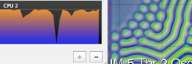
PDE4 on Core 2 Duo, with LogCPU load monitor
Most recently, in 2009 I revisited the project (mainly to set up this web site) and created the multi-threaded implementation for SMP (shared-memory parallel) systems. On a single node of a 2.33-GHz Intel Core 2 system it runs at 151 Mcgs; on an 8-core Xeon E5520 system it achieves just over 1800 Mcgs. (Perhaps even more impressively, a single thread running alone on the same Nehalem system achieves 275 Mcgs, almost double the Core 2's single-threaded speed). Memory speed does not factor into the comparison; the same ratios are seen when the dataset far exceeds the level-2 cache, as when it fits easily. (This is due to special care I have given to address the memory bandwidth bottleneck, see below). From the original PowerPC to a present-day machine of equal cost, I have seen a speed improvement of nearly 3000 over 15 years, a doubling in speed every 15.6 months. Double-precision performance is about half that of the figures quoted here, and this ratio has been about the same throughout the project's 15-year history.
I currently do most of my work on 512×512 grids (4× the area of the original Caltech grids) because it shows a greater variety of patterns and allows me to view a million tu in just a few minutes. Occasionally (such as when the parameter F is greater than about 0.05) I will let it run as much as an hour or two, or overnight when generating timelapse movies or a view of the full parameter map like that at the top of this page. Some tests have been run for as long as 4 months.
Some instructions for my own software are here: PDE4 User Manual. The program is for MacOS only. Here is a recent version: PDE4 2011 Oct 5. If you have trouble running this or have questions, contact me.
In the fall of 2010 I created a screensaver using OpenGL kernels to perform the reaction-diffusion calculations on the GPU. See my screen savers page for more details, screen shots, and to download the screensaver itself.

my face rendered in Gray-Scott
Optimising Reaction-Diffusion Simulations
My reaction-diffusion simulation work has been a long journey (18 years at this writing) of progressive optimization to adapt to new hardware. In the first 15 years, its performance increased by a factor of more than 3000, effectively utilising the hardware's full potential at all stages.
1994: The Caterpillar Scan
I began this project in 1994, just after the original Xmorphia website appeared. The standard algorithm at the time was forward Euler integration, (and my later studies showed that this is more than adequate for even the most complex Gray-Scott phenomena). Using the standard "ping-pong" method, one uses two grids (arrays) of data. With the gridsize that Pearson and Williams used, each grid would be 256×256×2×4 bytes, or 512 KiB, which amounts to 1 MiB total for the two grids.
In 1994 I had a 60 MHz PowerPC 601. This chip has a 32K unified L1 cache, and I had not installed the optional external 256K L2 cache. I discovered that with the 256×256 grids things ran at a speed that seemed reasonable, but with the larger grids I was trying to use for parameter space plots, performance fell sharply.
Since each grid cell is two single-precision floating point numbers, a row of 1024 cells consists of 8192 bytes of data, which is typically stored as two separate blocks of 4096 bytes. The Euler calculation requires reading three rows of input and writing one row of output; all of these rows get read into the cache on the first row scanned. For the cache to be useful, two of those input rows need to remain in the cache for when we calculate the second row. That means that four rows of data need to fit in the cache. So a grid width of 1024 cells would be trying to put 4×8 KiB = 32 KiB of grid data in the cache, and that won't fit because it's a unified cache: some of the cache is used up by the code (program instructions). A grid width of 1024 was extremely slow, and in fact I didn't get much over 512 before things got slow.
So the first optimization I used was what I called the "caterpillar scan", so-called because the data end up creeping along like the feet on a caterpillar that is walking forwards. We use just one grid, but we start by adding an extra row to the top and bottom of the grid — and on each row, the output (new values for that row) get written over the previous row. The processing of a single iteration of the whole grid goes like this:
|
Notice that the output is offset by one row from the input: that's because we always need the "old values" of the two neighboring rows when computing each new row: so when the new value of row N is written, it must be written over row N-1 so that the old value of row N is still available when working on row N+1. (During subsequenct iterations, the grid continues to creep down; modular arithmetic simplifies things a bit.)
Using the caterpillar algorithm the cache impact of the grid width was half as great, because there's only one grid: the row being overwritten is already in the cache. Here are my original PowerPC 601 benchmarks:
|
I was perfectly happy with this (the theoretical peak MFLOPs of this CPU is 120 MFLOPs, but that's only achievable without loads and stores. I did achieve 92 MFLOPs in my Power MANDELZOOM but only by keeping everything in registers.)
2004: GCC Compiler and Register Variables
By 2004 I had an 800 MHz PowerPC 7445 with 64K of L1 cache and 256K of L2 cache. My old PDE1 program had been built with MetroWerks CodeWarrior C++, and I created a new version (called "PDE2") in Xcode. But PDE2 failed to match the performance of PDE1. After some investigation I discovered that the new compiler (a version of GCC) was no longer putting local variables in registers, something CodeWarrior has been doing quite well. There are 32 registers of each type (float and integer) and at least half are available for use within a subroutine.
After some digging around and experimentation, I discovered that the solution for the GCC compiler was to declare local variables like this:
register real_type F ASM("f1"); register real_type dF ASM("f2"); register real_type u_u ASM("f3"); ...There was also a new way to tell it to generate FMA instructions (the -mfused-madd flag). With these changes, the newly compiled PDE2 matched the performance of PDE1:
|
2004: 128-bit Vector SIMD
The main reason for moving PDE1 to the new compiler was so that I could utilise the PowerPC 7445's "AltiVec" unit, a 128-bit-wide SIMD vector unit. It had the potential of delivering up to 4 times as many MFLOPs, although the need for additional data movement typically reduces the efficiency a bit.
I worked out a way to scan across a grid row 4 cells at a time, while keeping some of the data in AltiVec registers so that the next 4 cells don't have to re-load some of the needed input values. The result was a quite satisfactory improvement of about 3×:
|
2004: Cache Line Alignment Investigation
In the above two tables, I have highlighted the column with the highest performance. You might nitice that the results for a row length of 1024 cells is suspiciously low in the single threaded scalar results, and suspiciously high in the single threaded vector results.
I suspected this was because of "cache lines", and wrote my own version of the STREAM benchmark to investigate. I spent quite a while looking at the memory system performance of two 800 MHz PowerPC 7445 (with different types of memory) and worked out exactly how many cycles it takes to load each vector (128 bits or 16 bytes) of data. I eventually figured out three things:
- Due to the organization of the cache (8-way set-associative, 32-byte cache lines) certain row lengths will make the L1 and L2 caches behave as if they are much smaller than 64K and 256K respectively.
- In many cases performance is improved by interleaving the two floating-point values of each grid point so that all the data is in a single big array.
- Most grid sizes benefit from using the vec_dst (data stream touch) instruction, which tells the CPU to pre-load data that will be used soon.
Combining these techniques led to a substantial improvement, and with a more consistent performance for different row lengths:
|
2004: Millipede Scan
As part of the investigation of cache performance I worked out that I could achieve a greater cache hit rate by performing more than one "caterpillar scan" in parallel. This is easiest to visualise by imagining that there are two people going through the grid in parallel, with one "in the lead" and the other following just a few rows behind.
This requires adding more extra rows to both the top and bottom of the grid, because if we're going to compute 2 new generations, we need 2 extra rows on each side.
|
If you watch a real millipede walking, it's actually a lot like this: there are several places where the feet are off the ground, and these places travel like waves in the "backwards" direction while the while millipede moves forward. Our data move like this: we scan from the top down, but the result (generation 2 output) ends up two rows higher.
The practical benefit of this is greater cache locality: to compute two generations we only need to scan the whole grid once. As long as 6 rows of data can fit in the cache, the cache will only "miss" once per row.
I call this the zig-zag scan because of the order in which memory is being accessed. The above diagram represents a "double-interleaved" zig-zag scan, but it can be more than that. The optimum amount of "interleaving" depends on the size of the processor caches and the size of the grid being simulated.
As before, continued operation requires using modular coordinates and having the grid data "wrap around" to continually re-use a fixed amount of memory. Here are the results I got in 2004. For each different grid size, I use boldface to highlight which overscan value ran fastest:
|
2009: Multi-Threaded Implementation
I revisited the project in 2009, using a dual-CPU PowerPC "G5" system. To use multiple threads, the grid is divided into "stripes" with each stripe being computed by one thread. This is a common practice, but in our case the "stripes" do not remain fixed. For the "millipede scan" to work, the stripes have to move through memory in lock-step. Each thread is performing a millipede scan, and the millipedes march together around the (cylindrical) grid. After each O steps of calculation (where O is the "overscan"), each CPU surrenders 2O rows of memory to the jurisdiction of the CPU following it. Data transfer between threads is optimal, with each CPU sending only 2O rows and receiving 2O rows of data to/from its neighbors in the ring; Total memory usage for the entire grid is optimal, given the choice of "overscan" value. The entire model will typically fit in the shared L3 cache of the multi-CPU system. The design is optimal on a variety of CPU, cache and memory configurations.
|
2009: Intel Conversion
I then moved to an Intel Core 2 Duo. This required two major changes. I added a set of macros to hide the use of compiler intrinsics for vector operations. With my macros, which are available here, the same C source will work on PowerPC or Intel vector intrinsics and even in cases where neither are available.
I made additional changes to handle the "little-endian" storage of data in memory (which affects how vector loads and stores get 4 consecutive array elements, and matters if the array is also being accesses by non-vector code e.g. for drawing). Most of this was handled by the vector macros, which hide the fact that array element 0 is loaded into the lowest vector element on an Intel system, and into the highest element on a PowerPC system.
As compared to the dual 2.0 GHz PowerPC G5, The 2.33 GHz Core 2 Duo does about 40% better.
|
2009: 8-core Nehalem System
On my 8-core system I have 16 MB of L3 cache, which is enough to hold all of the grid data for grids up to about 1024x1024 pixels (with room to spare for code and everything else that needs to be cached). I created many long-term time-lapse videos, most on a 480x336 grid; it was easy to run two or three of these at the same time, using 4 or 8 threads per each simulation.
This is a dual Xeon E5520 system. Each CPU has 4 cores and runs at speeds from 2.27 GHz to 2.53 GHz depending on how many cores are active.
Using just 2 threads should give more "performance per thread" than with 4 threads or more, both due to Amdahl's Law and because each CPU will have just one active core, allowing the clock rate to go up to the maximim 2.53 GHz. Based on clock speed alone I would expect to get about 324 Mcgs at the large grid size. In contrast to the Core 2 Duo, on this dual Xeon system data needs to be transferred between the two CPUs throughout the test. However, any slowdown from that is greatly outweighed by the DDR memory controller being right on the CPU die, and other Nehalem microarchitecture improvements. Thus, the 2-thread benchmarks shown here actually exceed the 324 Mcgs estimate.
For these tests I changed the 300×300 and 600×600 grids to 296×304 and 592×608 respectively, because this makes the number of rows a multiple of 16, needed for the 16-thread benchmarks below.
|
To measure the impact of Amdahl's Law, I repeated almost every test using 4 threads, then again with 8 threads and finally with 16 threads (except for the smallest gridsize).
|
Due to resource contention between threads in Intel's "Hyperthreading", and because of the variable clock speed ("Turbo Boost"), one would expect 16 threads to complete a task no morer than 5 times as fast as 2 threads, even if the task involves no appreciable memory transfer (e.g. Mandelbrot calculations).
Here we achieved a ratio of 33.76/13.30 ~ 2.53 for the small 300×300 model, and 53.37/15.69 ~ 3.4 for the large 2400×2400 model.
In 2009 I prepared a scientific paper describing some of the more exotic patterns and my work to confirm or disprove their existence; see my formal scientific research page, and the figures and animations. I added corrections and in 2014 put it on arXiv.org at abs/1501.01990.
In 2010 I gave a talk in the Rutgers Mathematical Physics Seminar Series; the slides, links to videos, and associated notes are here: 2010 Rutgers talk
References
[1] A. M. Turing, The chemical basis of morphogenesis, Philosophical Transactions of the Royal Society of London, series B (Biological Sciences), 237 No 641 (1952) 37-72. (PDF at cba.media.mit.edu: Turing 1952)
[2] Jonathan B. L. Bard, A Model for Generating Aspects of Zebra and Other Mammailian Coat Patterns, Journal of Theoretical Biology 93 (2) (November 1981) 363-385.
[3] Hans Meinhardt, Models of Biological Pattern Formation, Academic Press, 1982.
[4] S. Wolfram, Universality and complexity in cellular automata, Physica D: Nonlinear Phenomena 10 (1984) 1-35.
[5] P. Gray and S. K. Scott, Autocatalytic Reactions in the Isothermal Continuous Stirred Tank Reactor, Chemical Engineering Science 39 (6) (1984) 1087-1097.
[6] Q. Ouyang and H. L. Swinney, Transition from a uniform state to hexagonal and striped Turing patterns, Nature 352 (1991) 610-612.
[7] K. J. Lee, W. D. McCormick, Q. Ouyang, and H. L. Swinney, Pattern formation by interacting chemical fronts, Science 261 (1993) 192-194.
[8] J. Pearson, Complex patterns in a simple system, Science 261 (1993) 189-192. (available at arXiv.org: patt-sol/9304003)
[9] K. J. Lee, W. D. McCormick, H. L. Swinney, and J. E. Pearson, Experimental observation of self-replicating spots in a reaction-diffusion system, Nature 369 (1994) 215-218. (PDF at chaos.ph.utexas.edu: Lee et al.)
[10] A. Doelman, T. J. Kaper, and P. A. Zegeling, Pattern formation in the 1-D Gray-Scott model, Nonlinearity 10 (1997) 523-563.
[11] C. B. Muratov and V. V. Osipov, Spike autosolitons in the Gray-Scott model, CAMS Rep. 9900-10, NJIT, Newark, NJ. (available at arXiv.org: patt-sol/9804001)
[12] Allen R. Sanderson et al., Advanced Reaction-Diffusion Models for Texture Synthesis Journal of Graphics, GPU, and Game Tools 11 (3) (2006) 47-71.
[13] Karl Sims, Reaction-Diffusion Tutorial (web site), 2013.
[14] Greg Cope, Reaction-Diffusion: The Gray-Scott Algorithm (web page), 2014.
[15] R. Munafo, Stable localised moving patterns in the 2-D Gray-Scott model (2014). On arXiv: abs/1501.01990. (figures; original 2009 draft).
Links
If your browser supports WebGL (see 10), you can experiment with the full diversity of patterns in the Gray-Scott system using my WebGL Reaction-Diffusion Explorer.

WebGL Reaction-Diffusion Explorer
The best standalone program for getting started with reaction-diffusion is Ready, a fast, easy to use and versatile reaction-diffusion explorer for Windows, Mac and Linux. There are downloadable working versions, and it's an open-source project.

U-skates in Ready
If you have a Mac (running "Snow Leopard" or later) you'll probably also appreciate my xmorphia PDE5 screensaver, which turns the webcam image (i.e. you!) into a continually evolving Gray-Scott pattern:
Xmorphia PDE5
The Abelson et al. applet 2 is a quick and easy way to experiment with Reaction-diffusion in your browser. It is a bit difficult to draw a pattern manually, but it is the only web-based simulator that supports different types of grids, and it doesn't require WebGL:

U-skates on a hex grid
Replicating my Patterns in Ready
The Ready program is quite versatile and has lots of options. so it can be a bit tricky to get started. Here is an example which replicates the "soap-bubbles" pattern at (F=0.090, k=0.059):
- In the Patterns pane, select "grayscott_2D.vti" (in the "CPU-only" section)
- In the Info pane, find "k 0.064" and click the blue "edit" link next to the 0.064. Change k to 0.059.
- Similarly, find "F 0.035" and change F to 0.09
- Change D_a to 0.2 and D_b to 0.1
- Change Dimensions to 128×128×1
- Click the green triangle ("play button") or select "Run" from the Action menu.
- After running the pattern briefly, stop it.
- Now use the eye-dropper and paintbrush tools to edit the "b" area. Sample the light blue blob, and paint almost the whole thing that colour. Leave just a few spots of dark blue.
- Use the Run command again to continue running the pattern.
- The dark blue spots you left will become "soap bubbles" as seen in this YouTube video.
Be patient. It takes several minutes on my computer to get nice hexagonal bubbles.
If your computer has a reasonably modern GPU you can use the "Pearson1993.vti" pattern file instead, and it will run faster. Change the instructions as follows:
- Set k and F as described above.
- Do not edit D_a, D_b, or Dimensions.
- In Info Pane, Render settings, next to "show multiple chamicals" click "edit" which will change the setting to "true" making b visible. Then use "Fit Pattern" in the "View" menu to see both a and b.
- Do the paintbrush work before you run the pattern.
- Now paint it mostly light-blue as I described above and run the pattern.
Other Online Resources
1 : Jonathan Lidbeck has created this Java applet with extensive presets, options and instructions. He also provides a 3-D version. (Old URLs were http://ix.cs.uoregon.edu/~jlidbeck/java/rd/ and .../java/rd/3d.php)
2 : A group (Abelson, Adams, Coore, Hanson, Nagpal, Sussman) at MIT have created this website showing Gray-Scott pattern phenomena in grids of points that are connected "amorphously", more closely modeling how things would happen in a biological system of living cells.
3 : The original Xmorphia website is preserved by archive.org. View its December 1998 incarnation here.
4 : My paper is here and the slides from the talk I gave in 2010 are here.
5 : I also have pages on (deterministic quantised) cellular automata.
Footnotes
6 : Why UV2? : This is due to the so-called law of mass action (in its kinetic aspect), the fundamental relationship between stochiometry and reaction rate that generally applies when all reagents 8 are free to move around and participate in any available reaction. The value UV2 results from the facts that the odds of finding a molecule of U at any given place are proportional to the concentration u=[U], and in order for the reaction to take place you need to have one U and two V's in the same place at the same time. This ignores the rate constant, reverse reaction, and many other details: the reaction-diffusion model above has been simplified by converting to dimensionless units, ignoring any heat, ionization, association, etc. considerations, leaving just UV2. The law of mass action is a fairly rare example of a place in applied mathematics where addition and multiplication become multiplication and exponentiation respectively ("U plus V times 2" becomes "u times v to the power of 2") 7. It is because of this transformation, particularly the exponentiation part, that certain substances such as pure oxygen are so dangeous: when you increase the concentration from, say, 5% to 50%, the reaction rate of an otherwise rare reaction of the form "4O2 + A ... → B + ..." increases by a factor of 10,000.
7 : Multiplication to exponentiation : I love stuff like this, see my large numbers pages if you have any doubt.
8 : or "reactants".
9 : Names for the k parameter include "decay" or "poisoning" rate (Gray and Scott, 1984 [5]), "dimensionless rate constant of the [V→P] reaction" (Pearson 1993 [8]), "degrading rate" (Sanderson 2006 [12]), "conversion" [of V to P] (Abelson et al. 2009 2), "kill rate" (Karl Sims 2013 [13]), "removal rate" (Greg Cope 2014 [14]).
10 : The WebGL explorer requires a little more than just basic WebGL: framebuffer_object and texture_float. It should work in all major desktop browser versions since 2014.
This page was written in the "embarrassingly readable" markup language RHTF, and was last updated on 2022 Jun 20.
 s.27
s.27