Successive Refinement

Robert P. Munafo, 2023 Aug 20.

Successive refinement is an algorithm for graceful gradation in rendering, image processing, and other generally grid-oriented compute-intensive operations. It is particularly useful in interactive systems because of its presentation of coarse intermediate results to the user. In certain algorithms it can form the basis of optimizations which take advantage of local similarity, local common subexpressions, local linearity, or some similar phenomenon.

Successive refinement algorithms vary, but the common principle is to scan the grid at a "coarse" spacing, then again (in one or several passes) at increasingly finer spacings. To give two examples:

DEMZ subdivides pixels by a factor of two each time (8x8 squares, 4x8 rectangles, 4x4 squares, ...) with each stage centred on the location of the point being iterated, resulting in a staggered or offset tiling effect. See an example image below.

FRACTINT refers to their implementation as "diffusion scan", and subdivides squares into four smaller squares, but performs three passes at each level, filling in pixels in an ordering like that of ordered dithering.

Successive refinement is used in fractal programs as both a user interface device and as a speed optimization. The improvement that it provides cannot be overemphasized. It will instantly transform a barely useable program into a powerful viewer. If the successive refinement implementation includes the solid guessing adjacency optimization, the program will complete its work typically 2-3 times faster. With or without adjacency optimization, a usable image (suitable for navigating, e.g. selecting a sub-area for the next zoom) is often a hundred times faster — this is because the lower-resolution yet complete image visible early on allows the user a glimpse of the final result, often foregoing the need to wait for completion. The source code below shows how to do both versions, starting with a simpler non-solid-guessing version.

After first pass (1.5 sec.)	After second pass (4.5 sec.)
After third pass (13 sec)	After fourth pass (38 sec)

Four stages of successive refinement, with actual total elapsed times, as implemented by Super MANDELZOOM (1985), my first Mandelbrot viewer program. The image is the same as that on the August 1985 Scientific American cover.

Successive Refinement as a User Interface Improvement

As a user interface device, successive refinement allows the user to view a coarse representation of the current image, followed soon after by a less coarse version, then by better and better versions gradually over time. The implementation is fairly simple, consisting of little more than several successive raster scans. This can be done as follows:

Program MANDELBROT-SR-1 ~~~~~~~~~~~~~~~~~~~~~~~ COMMENT "The crudest Successive Refinement algorithm, applied to the Mandelbrot Set. Allows the user to quit early if the coarse rendition shows that the image will be uninteresting." FOR chunk_size IN {16, 8, 4, 2, 1} DO FOR x = 1 TO grid_width INCREMENT_BY chunk_size DO FOR y = 1 TO grid_height INCREMENT_BY chunk_size DO LET r = XtoRealCoord(x) LET i = YtoImagCoord(y) LET count = EscapeIterations(r,i) LET color = MyColorMapping(count) FillRectangle(PARAM("left") = x, PARAM("top") = y, PARAM("width") = chunk_size, PARAM("height") = chunk_size, PARAM("color") = color) IF UserIntervention() THEN EXIT FOR(chunk_size) END IF END FOR(y) END FOR(x) END FOR(chunk_size)

On each iteration of the outermost FOR loop, the grid is scanned, evaluated, and plotted in squares of the current chunk size. The subroutine "fill_rectangle" takes five parameters, as shown: the top-left coordinates, the width and height, and a color.

This implementation is of course slower in the end than a single grid scan, because 25% of the squares are iterated and drawn twice, and 6.25% are drawn three times, etc.

With fairly little effort we can avoid this extra computation.

Program MANDELBROT-SR-2 ~~~~~~~~~~~~~~~~~~~~~~~ COMMENT "Successive Refinement, avoiding repetition of work done on the previous pass." FOR chunk_size IN {16, 8, 4, 2, 1} DO FOR x = 1 TO grid_width INCREMENT_BY chunk_size DO FOR y = 1 TO grid_height INCREMENT_BY chunk_size DO IF ( chunk_size EQUALS 16 ) THEN LET do_evaluate = TRUE ELSE IF ( ((x / chunk_size) DIVISIBLE_BY 2) AND ((y / chunk_size) DIVISIBLE_BY 2) ) THEN LET do_evaluate = FALSE ELSE LET do_evaluate = TRUE END IF IF ( do_evaluate ) THEN LET r = XtoRealCoord(x) LET i = YtoImagCoord(y) LET count = EscapeIterations(r,i) LET color = MyColorMapping(count) FillRectangle(PARAM("left") = x, PARAM("top") = y, PARAM("width") = chunk_size, PARAM("height") = chunk_size, PARAM("color") = color) IF UserIntervention() THEN EXIT FOR(chunk_size) END IF END IF END FOR(y) END FOR(x) END FOR(chunk_size)

Inside the three loops we have added two tests. The first ensures that the first scan (chunk_size 16) will be complete. The second allows subsequent passes to skip the squares computed on the previous pass.

Successive Refinement as a Performance Optimization

Optimization via Successive refinement is a little more difficult, but well worth the effort. The technique is to watch the neighboring points during the grid scan and skip the Mandelbrot iteration if all of the neighbors have the same "count". This works quite well for the Mandelbrot Set (at least at the low magnifications that most beginning explorers use — see Optimizations - Domains of Efficacy)

Program MANDELBROT-SR-3 ~~~~~~~~~~~~~~~~~~~~~~~ COMMENT "Successive Refinement for the Mandelbrot Set, with optimization to take advantage of local similarity (solid regions)."

Implementation starts by declaring an array to hold the computed count values :

DECLARE counts_array: ARRAY[1 TO grid_width, 1 TO grid_height] OF INTEGER

Our three loops are the same :

FOR chunk_size IN {16, 8, 4, 2, 1} DO FOR x = 0 TO (grid_width-chunk_size) INCREMENT_BY chunk_size DO FOR y = 0 TO (grid_height-chunk_size) INCREMENT_BY chunk_size DO

We compute the coordinates of the current square's "parent". These are the coordinates of the square from the previous pass that the current square is a part of. For example, on the second pass, the square at (8,24) is an 8x8 square which is a part of the 16x16 square at (0,16). Thus (0,16) are the coordinates of the "parent" of (8,24).

IF (x DIVISIBLE_BY (2*chunk_size)) THEN LET parent_x = x ELSE LET parent_x = x - chunk_size END IF

The computation of parent_y is similar :

IF (y DIVISIBLE_BY (2*chunk_size)) THEN LET parent_y = y ELSE LET parent_y = y - chunk_size END IF

We then perform a test to see if the current square should be evaluated. The first part of the IF ensures that all squares will be drawn on the first pass, just as before :

IF ( chunk_size EQUALS 16) THEN LET do_evaluate = TRUE

The second part, just as before, ensures that we skip squares that were drawn on the previous pass — note however that the test is now simplified because we can use the variables parent_x and parent_y :

ELSE IF ( (x EQUALS parent_x) AND (y EQUALS parent_y) ) THEN LET do_evaluate = FALSE

The third part is the new test : it calls a subroutine, "all-neighbors-same", which will return TRUE if all of the neighboring squares have the same count as the square given by the parameters parent_x and parent_y. "chunk_size * 2" is the spacing between the parent square and the neighboring parent squares. Eight neighbors will be tested :

ELSE IF (all-neighbors-same(parent_x, parent_y, chunk_size * 2) ) THEN LET do_evaluate = FALSE

The last part of the IF is the default : if none of the other tests worked, we must evaluate the point :

ELSE LET do_evaluate = TRUE END IF

After determining if we evaluate, we then proceed as follows :

IF (do_evaluate) THEN LET r = XtoRealCoord(x) LET i = YtoImagCoord(y) LET count = EscapeIterations(r,i) ELSE LET count = counts_array[parent_x, parent_y] END IF b

This instructs the computer to use the "parent"'s count value if we are on a square that is being skipped. Then we proceed to draw :

LET counts_array[x,y] = count LET color = MyColorMapping(count) FillRectangle(PARAM("left") = x, PARAM("top") = y, PARAM("width") = chunk_size, PARAM("height") = chunk_size, PARAM("color") = color) IF UserIntervention() THEN EXIT FOR(chunk_size) END IF

This is the same as before, the only difference being that we store our count value in the array for use on the next pass. (Sharp readers will note that when a square has the same coordinates as its parent, we redraw it. This is of little consequence.) Now we end our loops :

END FOR(y) END FOR(x) END FOR(chunk_size)

As a user-interface improvement, successive refinement can work even better if the pixels are split in two (vertically or horizontally on alternating passes) instead of in four. In other words, if the first pass produces 8x8 pixels, the second would produce 4x8 pixels, the third 4x4 pixels, the fourth 2x4 pixels and so on. Try out the JavaScript-based DEMZ viewer to see what this is like.

While these pseudo-code examples have used the Dwell or Escape-Iterations function for rendering the Mandelbrot Set, successive refinement lends itself equally well and with similar results to the Distance Estimator function.

With great effort, successive refinement can be applied to the Synchronous Orbit algorithm. Other perturbation methods such as differential estimation can do successive refinement with no more effort than with a standard non-perturbation iteration method.

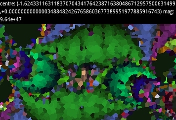
Use of Non-Square 'Pixels'

Successive refinement can be done with 'grids' other than evenly-spaced rows and columns, and with 'pixel' shapes other than square or rectangle. For example, a reader created a viewer that uses Voronoi cells as 'pixels'. The first image shows an intermediate stage in the calculation. The order in which individual points are evaluated is chosen quasi-randomly, from locations on an evenly-spaced grid, and making sure not to do any point twice.

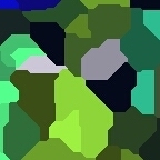
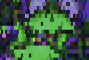
Successive refinement with Voronoi cells	The Manhattan distance metric was used
Using DEMZ-style chunky pixels	Completed image with DEMZ

(The two images in the second row are recreated in DEMZ, with somewhat different colours.)

revisions: 20100225 oldest on record; 20230803 add Voronoi section; 20230808 examples of SR variants; 20230809 contrast between SR with vs. without solid guessing; 20230820 images for Voroni and DEMZ methods

Mu-ency main page — index — recent changes — DEMZ

This page was written in the "embarrassingly readable" markup language RHTF, and was last updated on 2023 Aug 21.

s.27