Pearson's Classification (Extended) of Gray-Scott System Parameter Values

key map
Links to descriptions: alpha (α) beta (β) gamma (γ) delta (δ) epsilon (ε) zeta (ζ) eta (η) theta (θ) iota (ι) kappa (κ) lambda (λ) mu (μ) nu (ν) xi (ξ) pi (π) rho (ρ) sigma (σ)
(If you prefer the more universal Wolfram taxonomy, view the page Universality-Complexity Classes for PDE Systems)
The first fourteen (R, B, and alpha through mu) were defined by Pearson [1]; here are the data from his figure 3 (with corrections) replotted on the index image from the main page:
")
Pearson's labels (corrected)
Pearson missed many types of patterns because he only used one starting pattern: a small (u, v) = (1/2, 1/4) square on an otherwise (1, 0) background. Many combinations of paramters (F, k) fail to produce a pattern if initialised this way, but produce patterns when started some other way (such as a single small spot on an otherwise (0, 1) background, resembling the inverse of Pearson's initialisation; or several spots of diverse (F, k) values). Types nu, xi, pi, rho, and sigma are of this sort and were identified by me; the first three of these are described in my paper [2]. Types rho, and sigma also require a model with somewhat higher reqolution than Pearson's, and significantly better runtime; these requirements would have made their discovery nearly impossible in the 1990s. All pattern types are described here, each with links to specific examples that include still images and video.
Each pattern type can be differentiated from the others by looking at key properties such as oscillation, spot shape, system-wide determination vs. local determination (e.g. Wolfram class 2 vs. Wolfram class 3), etc. For Gray-Scott systems specifically, I usually use the first two (oscillation and spot shape).
The Two Parameters F and k
Karl Sims outlines the Gray-Scott equations with great illustrations starting with the idealised reaction of molecules that diffuse at varying rates. He describes the parameters F and k as "feed rate" and "kill rate".
Feed-Rate Spectrum: Stability/Oscillation/Chaos
Varying the parameter F while keeping k constant causes the system to move vertically in the parameter map at the top of this page. Varying k in such a way as to follow the "crescent-shaped" contour will reveal a spectrum of phenomena distinguished by the amount and type, if any, of oscillation.
|
Kill-Rate Spectrum: Soliton Type and Shape
Varying just the parameter k while keeping F constant reveals a second spectrum distinguished by the presence or absence of large solid regions, stripes, and/or spots. This spectrum does not appear in the lower F values where the system is too chaotic.
|
Pearson (and Munafo) Classes
These distinctions don't all work perfectly: for example the "negative stripes and spots but no positive spots" and its complement are contradicted by type rho and type sigma, in each of which the paradoxical spot expands to form bubbles demarcated by stripes; these happen up in the high-F region and have much slower evolution than, say, type epsilon
Nevertheless, we can combine the two distinctions into a two-dimensional arrangement, and organise the classes approximately like so:
|
Type R
Evolves to a uniform red state.
Type R patterns belong to Wolfram class 1.
Examples: (F=0.014, k=0.057), (F=0.074, k=0.069).
Type B
Evolves to a uniform blue state (possibly after a brief period of pattern-formation and/or oscillation resembling another type, such as β).
Type B patterns belong to Wolfram class 1.
Examples: (F=0.050, k=0.059), (F=0.078, k=0.059).
Type alpha (α)
Spatial-temporal chaos composed mainly of wavelets and "fledgling spirals" that repeatedly grow and/or multiply and quickly annihilate upon hitting another object.
Type epsilon (ε) differs from this by supporting rings, spot mitosis, and longer-lived clumps of spots.
Type α patterns belong to Wolfram class 3.
Examples:
 (F=0.010, k=0.047) | 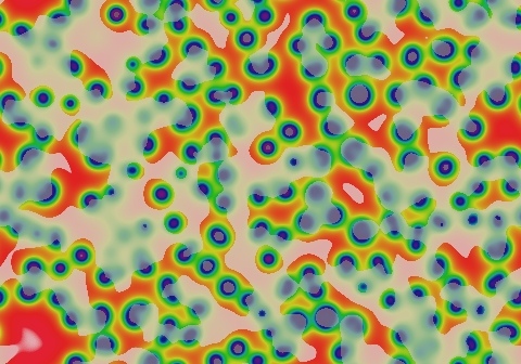 (F=0.014, k=0.053) |
Type beta (β)
Spatial-temporal chaos with localised red and blue state in different spots at different times. This looks like waves on a blue ocean with periodic red "voids" that open up suddenly and then quickly fill in with blue.
Type β patterns belong to Wolfram class 3.
Examples:
 (F=0.014, k=0.039) | 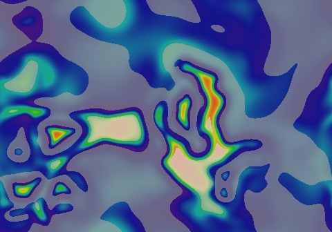 (F=0.026, k=0.051) |
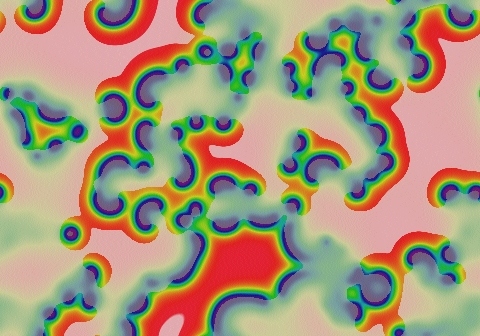
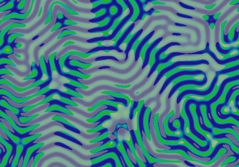
Type gamma (γ)
Stripes, either wormlike or branching, with endless instability in the form of occasional changes due to overcrowding, grain boundary instabilities, or other localised events, and oscillation in the ∂u/∂t component.
Type theta (θ) differs from this by having few or no die-out events and the oscillation in ∂u/∂t eventually ends.
Type γ patterns belong to Wolfram class 3.
Examples:
 (F=0.022, k=0.051) | 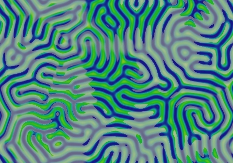 (F=0.026, k=0.055) |
Type delta (δ)
Includes true Turing patterns and many parameter values that produce similar patterns through a presumably related effect.
The true Turing pattern arises from a starting pattern that is all blue, with arbitrarily small noise or other irregularities.
In "Turing-similar" systems, a pattern cannot arise from an all-blue starting state, instead they need to be "seeded" by a large amplitude disturbance (anything non-blue and at least as large as a typical negaton will usually suffice); and the pattern grows outward from the disturbance.
In either case, the resulting pattern is a hexagonal array of negative spots, possibly with some stripes in place of rows of spots, and with grain boundaries that are asymptotically stable.
Type δ patterns belong to Wolfram class 2-a.
Examples:
 (F=0.030, k=0.055) | 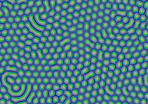 (F=0.042, k=0.059) |
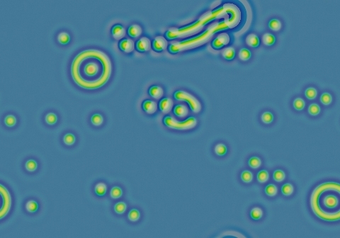
Type epsilon (ε)
Spatial-temporal chaos composed mainly of spots (resembling solitons but unstable). Rings can grow until they contact something else; spots with less symmetry tend to live longer and split via mitosis. Spots continually crowd each other out; after regions are opened up by die-outs; other spots on the boundary of the newly opened region quickly fill it in again.
Type alpha (α) differs from this by having no rings or symmetrical (round) spots.
Type lambda (λ) differs from this by having no overcrowding or die-outs.
Type zeta (ζ) differs by having spots that are somewhat less volatile, reproducing in a more symmetrical way and being more long-lived, though die-outs still occur.
Pearson [1] misidentified two tests as type ε: the parameters (F, k) = (0.025, 0.0625) and (0.03, 0.0625) both yield type lambda (λ) behaviour.
Type ε patterns belong to Wolfram class 3.
Examples:
 (F=0.018, k=0.055) | 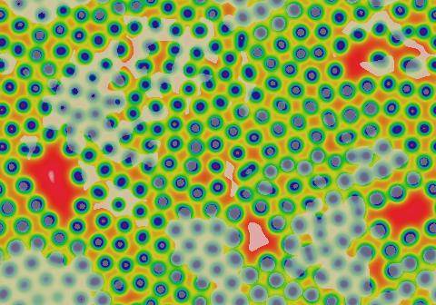 (F=0.022, k=0.059) |
Type zeta (ζ)
Very similar to type epsilon (ε), but viable spots are generally more symmetrical and more stable, and the disturbances that cause spots to die are limited to a smaller percentage of the domain at any given time. In some ζ patterns these areas of disturbance travel slowly rather than appearing suddenly at random. There is also a subtle oscillation (seen in the ∂u/∂t component in the examples).
Type epsilon (ε) has more volatile spots and constant overcrowding die-outs; type lambda (λ) has no die-outs at all.
Type ζ patterns belong to Wolfram class 3.
Examples:
 (F=0.022, k=0.061) | 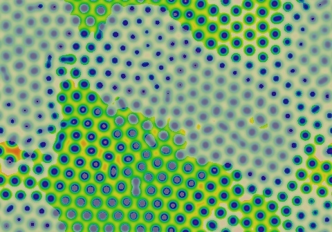 (F=0.026, k=0.059) |
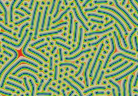
Type eta (η)
Similar to type gamma (γ), but instead of all stripes there is a mixture of spots and worms. Any longer or more serpentine stripes will break up into short pieces. Ongoing activity includes low-level oscillation seen in the ∂u/∂t component, and spots occasionally splitting off and/or rejoining the worms; but the system always reaches a steady state if run for longer than the 200,000 tu in Pearson's experiments [1].
Type gamma (γ) differs from this by never reaching stability.
Type theta (θ) differs from this by having negative spots and stripes, rather than positive.
Type kappa (κ) differs from this by being mostly stripes/worms, including long and/or convoluted stripes, and by having no oscillation in the ∂u/∂t component or by settling down to a steady state more quickly.
Type mu (μ) differs from this by having no oscillation in the ∂u/∂t component, and almost no spots/solitons.
Type η patterns belong to Wolfram class 3.
Example:
 (F=0.034, k=0.063) |
Type theta (θ)
Blue spots grow into concentric rings; stripes in isolation grow width-wise into parallel or crosswise stripes. Final state is mostly all stripes (sometimes with a few solitons), usually with branching and can be fully connected (network of loops). At lower F values there can be long-lasting oscillation in the ∂u/∂t component, or the system might never stop changing.
Type gamma (γ) differs from this by having die-out events and unending oscillation in ∂u/∂t.
Type kappa (κ) differs from this by having no stable blue state, and stripes that are less likely to join.
Type eta (η) differs from this by having positive rather than negative spots and stripes.
Pearson [1] misidentified one test as type θ: the parameters (F, k) = (0.03, 0.059) actually yield something like type gamma (γ) but with no die-out events.
Type θ patterns belong to Wolfram class 2-a.
Examples:
 (F=0.030, k=0.057) | 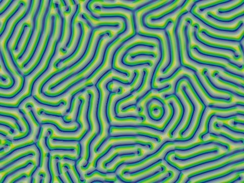 (F=0.038, k=0.061) |
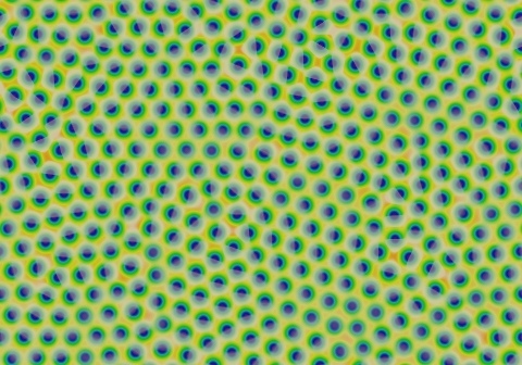
Type iota (ι)
Negative spots (negatons) with molecule-like interaction; solitary negatons are not viable.
This pattern class is closely related to type pi (π), which also supports linear and other shapes.
Type ι patterns belong to Wolfram class 2.
Example:
 (F=0.046, k=0.0594) |
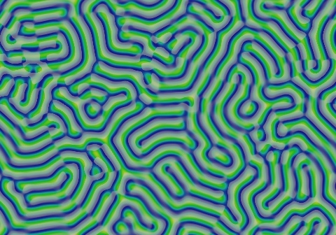
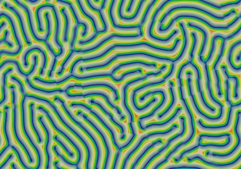
Type kappa (κ)
Stripes in isolation grow width-wise (usually by developing meanders to grow longer and more serpentine); some irregular blue shapes grow into corals. The final state is mostly all stripes, often with branching, and usually in multiple disjoint sets (hedgerow mazes).
Type theta (θ) differs from this by having a stable blue state, and stripes that are more likely to join.
Type mu (μ) differs from this by the fact that small blue spots turn into a worm, rather than growing out in all directions to form a ring or coral.
Type eta (η) differs from this by having shorter stripes/worms and many solitons, and oscillation in the ∂u/∂t component.
Type κ patterns belong to Wolfram class 2-a.
Examples:
 (F=0.050, k=0.063) | 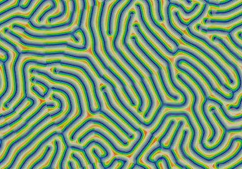 (F=0.058, k=0.063) |
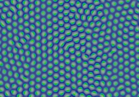
Type lambda (λ)
Solitons that grow by mitosis (cell-division). After the space is filled, solitons rearrange into hexagonal grids, sometimes with grain boundaries. Eventually, all movement stops and the pattern is in a steady state.
Type epsilon (ε) differs from this by having "overcrowding" and die-outs, and never reaching a steady state.
Types eta (η), theta (θ), and mu (μ) differ from this by having stripes.
Type λ patterns belong to Wolfram class 2-a.
Examples:
 (F=0.026, k=0.061) | 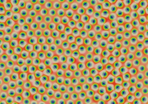 (F=0.034, k=0.065) |
Type mu (μ)
Stripes that grow from each end (worms), possibly also co-existing with inert (non-mitotic) solitons. After the space is filled by the worms, they reorganise towards parallel stripes and remain disconnected from one another.
Type eta (η) differs from this by having oscillation in the ∂u/∂t component, and many spots/solitons.
Type kappa (κ) differs from this by having branching and no solitons, and small blue spots grow into a ring or coral rather than a worm.
Type μ patterns belong to Wolfram class 2-a.
Examples:
 (F=0.046, k=0.065) | 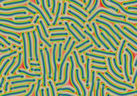 (F=0.058, k=0.065) |
For my paper [2] and talk [5] I added the following classes that are not in Pearson [1] :
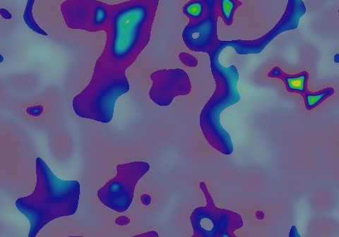
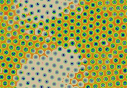
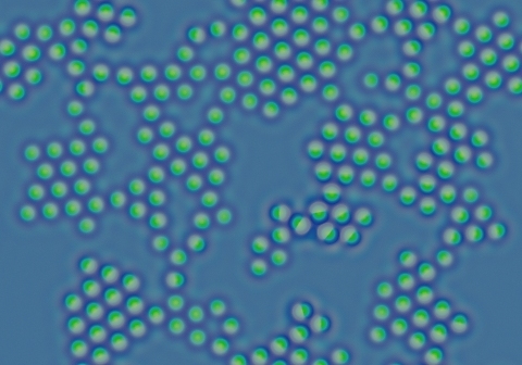
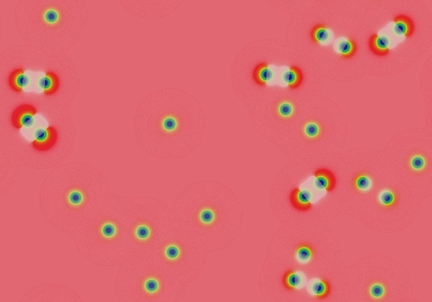
Type nu (ν)
Inert (non-mitotic) solitons. The number of solitons depends on the number and size of blue areas in the starting pattern. All large blue areas shrink and/or split up into solitons. The solitons then drift apart from each other to spread as uniformly as possible across the space, but this takes a period of time proportional to eKw where w is the width of the domain in lu and K is a constant, K≈20+1000F. In the following images (with F=0.046, k=0.067) each successive image represents approximately twice as much elapsed time:
 t=76 tu |  t=153 tu |  t=306 tu |  t=612 tu |
 t=1224 tu |  t=2448 tu |  t=4896 tu |  t=9792 tu |
 t=19584 tu |  t=39062 tu |  t=78125 tu |  t=1.5625×10⁵ tu |
 t=3.125×10⁵ tu |  t=6.25×10⁵ tu |  t=1.25×10⁶ tu |  t=2.5×10⁶ tu |
 t=5×10⁶ tu |  t=1×10⁷ tu |  t=2×10⁷ tu |  t=4×10⁷ tu |
 t=8×10⁷ tu |  t=1.6×10⁸ tu |  t=3.2×10⁸ tu |  t=6.4×10⁸ tu |
In the last frame the solitons have stopped only because double-precision arithmetic is no longer adequate to accurately compute u+∂u.
Type ν patterns belong to Wolfram class 2.
More examples:
 (F=0.054, k=0.067) |  (F=0.082, k=0.063) |
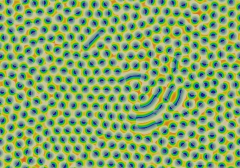
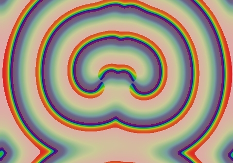
Type xi (ξ)
Large, sustained spirals similar to the Belousov-Zhabotinsky reaction in a Petri dish. The seed of the spiral is an essential and sometimes rare feature, which must exist in suitable quantities to produce a long-lived pattern. This means that if the domain is small, the spirals will die out; in this case the pattern becomes uniform red state. If the domain is large enough, occasional irregularities usually geerate new spiral seeds and thereby maintain the population of spiral seeds.
Type ξ patterns belong to Wolfram class 3.
Examples:
 (F=0.010, k=0.041) | 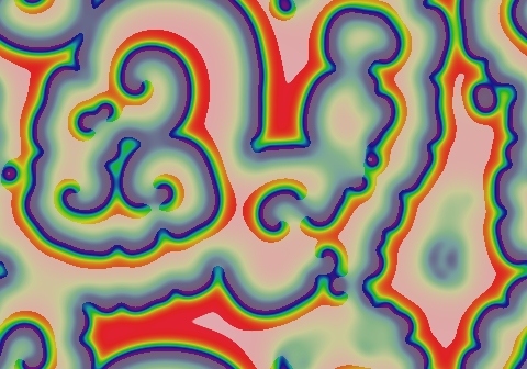 (F=0.014, k=0.047) |
Type pi (π)
Type pi supports stripes, loops, and spots, all of them negative. These form stable localised structures, both stationary and moving, and localised force-like interactions whose nature (attractive or repelling) oscillates in sign with increasing distance and whose strength decreases exponentially with distance. The combination of this force interaction and motion means that you also get rotating patterns.
Most significantly, the type pi patterns display such a great diversity that it is impossible to characterise the final outcome of a system just by looking at its initial state, except for a limited class of starting states (e.g. when the starting pattern consists only of lone negatons separated by large distances).
|
One specific example occurs at F=0.06, k=0.0609. I have explored this region extensively and written a paper which can be found here. There is also a catalog of patterns, several additional animations, and some discussion here.
Type π patterns belong to Wolfram class 4 (and possibly 4-a).
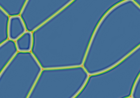
Type rho (ρ)
Systems that are blue except for a small number of negatons evolve into a set of closed red "soap bubbles" bordered by stripes exhibiting "surface tension". These usually combine in a manner resembling real-world soap bubbles, with smaller bubbles shinking and vanishing whilst neighboring larger bubbles grow (though in limited cases at certain parameter values a negaton can persist).
This behaviour is just like type sigma (σ) with red and blue reversed. However, "worm tips" (lines that end without joining with another line) sometimes persist or lengthen until they are constrained by the size of their containing bubble; in type σ such tips always shrink.
Type ρ patterns belong to Wolfram class 2-a.
Examples:
 (F=0.090, k=0.059) | 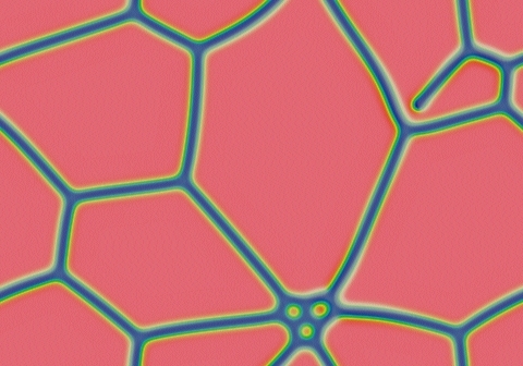 (F=0.102, k=0.055) |
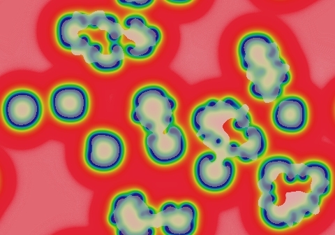
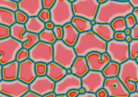
Type sigma (σ)
Systems that are red except for a small number of spots evolve into a set of closed blue "soap bubbles" bordered by red negative stripes exhibiting "surface tension". These bubbles usually combine in a manner resembling real-world soap bubbles, with smaller bubbles shinking and vanishing whilst neighboring larger bubbles grow (though in limited cases at certain parameter values a soliton can persist).
This behaviour is just like type rho (ρ) with blue and red reversed. However, "worm tips" (lines that end without joining with another line) always shrink; in type ρ such tips sometimes persist or lengthen.
Type σ patterns belong to Wolfram class 2-a.
Examples:
 (F=0.090, k=0.057) | 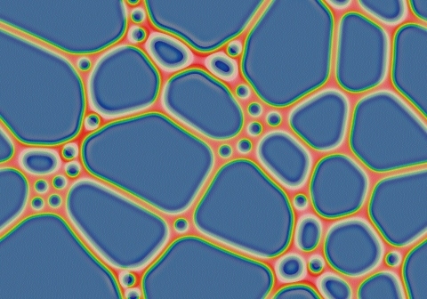 (F=0.110, k=0.0523) |
Back to main menu.
References
[1] J. Pearson, Complex patterns in a simple system, Science 261 (1993) 189-192. (available at arXiv.org: patt-sol/9304003)
[2] R. Munafo, Stable localized moving patterns in the 2-D Gray-Scott model (2009) 2009 draft (PDF) and figures ;
[3] 2010 revision (PDF) with the same figures ;
[4] 2014 revision on arXiv: abs/1501.01990
[5] R. Munafo, presentation on [2] delivered to the Mathematics department at Rutgers, 2010 Dec 9. text with illustrations, slides only: PDF, PPS
This page was written in the "embarrassingly readable" markup language RHTF, and was last updated on 2022 Mar 18.
 s.27
s.27