Exponential Map

Robert P. Munafo, 2023 Aug 8.

Coordinates can be transformed between polar and orthogonal in a mathematically natural way by using the complex exponential and logarithm functions. Both are Conformal maps which means that relatively small features have the same shapes after the transformation.

An exponential coordinate transformaion can be applied to a Mandelbrot or Julia view to give additional insight into its structure — in particular, showing structural similarities that exist over widely varying distance scales.

Here is an ordinary zoom sequence:

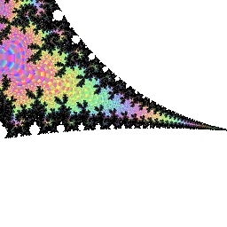
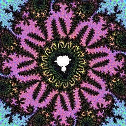
Center: -0.128219857864 +0.839741062363 i; size ranges from 2.0 down to 2.0×10^-8 in successive powers of 10

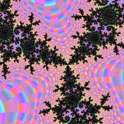
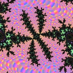
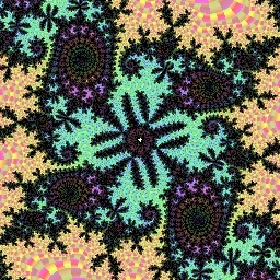
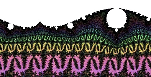
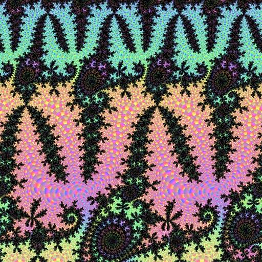
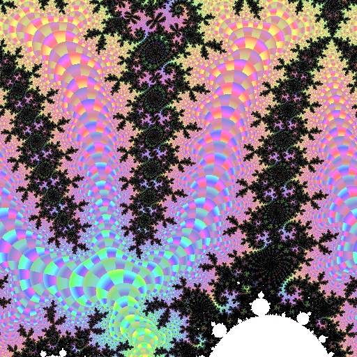
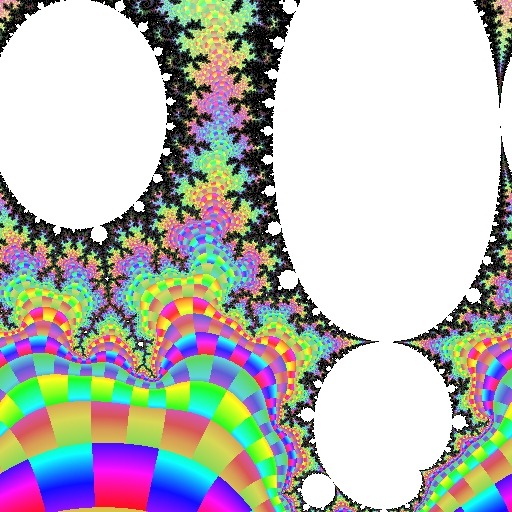
And here is the same location in the Mandelbrot set viewed through an exponential map:

There is another example in my Leavitt navigation description, and this other example, both are from 2010.

Identities

Some things to note about exponential maps:

The exponential mapping transforms the entire complex plane into a strip that has unlimited length along the real axis, and a width of 2π along the imaginary axis. (In the example shown here, the width is 512 pixels from left to right: I rotated the strip 90^o to make it run vertically down the page.)

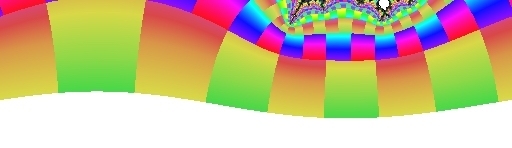
Circles that are centered on the point of interest become horizontal lines in the transformed image. Offset circles turn into a sort of sinewave (one can be seen at the bottom edge of the example image).

Spirals that are centered on the point of interest become diagonal lines in the transformed image.

In the vertical direction, a distance of 1.0 corresponds to a distance ratio of e=2.7182... in the original coordinates. (In the example shown here, 2π is 512 pixels, so one unit is 256/π = 81.49 pixels. When you move that far down in the image, you are moving 2.7182... times as far away from the central point -0.128219857864 + 0.839741062363i)

The left and right edges of the strip correspond to east (the direction in which the real coordinate increases, commonly depicted as being towards the right) in the normal coordinate space. (Thus, the right edge slices through R2.1/3.1/2a because you pass through that mu-atom if you start at -0.128219857864 + 0.839741062363i and move in the increasing real direction.)

The center line of the strip (midway between the left and right edges) corresponds to west (the direction in which the real coordinate decreases, commonly depicted as being towards the left) in the normal coordinate space. (Thus, the tip R2t, also called the spike, is found near the center at the bottom-most end of the strip image)

Vertical lines 1/4 and 3/4 of the way from the strip's left edge to its right edge correspond to north and south respectively. (In the image, the period-4 island R2F(1/3B1)S is at about the 1/4 point because it is located "north" of -0.128219857864 + 0.839741062363i. The cusp R2.C(1/3) is about 3/4 of the way across because it is "south" of -0.128219857864 + 0.839741062363i, and a tiny R2.2/3a can be seen below that.)

Circular mu-atoms appear as "ellipses" (they are not really ellipses, both because the logarithm function is nonlinear and because the mu-atom itself is not a perfect circle). The "eccentricity" is related to the ratio between the distance from the center point to the mu-atom and the radius of the mu-atom. Thus, mu-atoms that are large in comparison to their distance from the center-point appear as more eccentric "ellipses". The long axis is always vertical. (In the example image shown here, the largest mu-atom is R2.1/3a. It appears to the right of the centerline because it is to the south of the center coordinate of the area of interest.)

Cardioid (seed) mu-atoms are similarly transformed.

Repeating features created by the self-squaring action of the influencing island appear as identical units, tiled in a binary cascade (a self-simlar tesselation). Similar tesselations are seen near the edges of the M. C. Escher work Square Limit. (In normal coordinates, these repeated features appear more like an inside-out version of Escher's Circle Limit III).

Optimization for Zoom Animations

If rendered at suitable resolution, and using bilinear interpolation, an exponential strip image can be used as source data for rendering frames of a Mandelbrot zoom animation. An inverse mapping (using the complex logarithm function) is used to compute the location (in the strip) of needed data for any given location in the normal orthogonal coordinate space.

This is an almost ideal speed improvement: all features will be rendered at exactly the resolution needed for the zoom animation, and no Mandelbrot iterations get computed twice.

History

I discovered the utility of this coordinate transform in April 2002 while searching for the "Polaftis" image (see Reverse Bifurcation) of Jonathan Leavitt.

Locating images like "Polaftis" is an esoteric learned skill, which I call Leavitt navigation. A person can do it without using exponential map views, but it is harder. It is also immensely more difficult to take a "mystery image" found online and figure out how to find it (or anything with a superficially similar structure).

C Source Code

Given this setup code to define the view boundaries and related values:

Compute values that are common to every pixel calculation in a view /* Inputs are: ctr_r is the real coordinate of the center of the view we want to plot ctr_i is the imaginary coordinate of the center of the view real_width is the width of the image (in real coordinates) this should reflect the width when "zoomed in" all the way pixel_width is the number of pixels per row of the image we want to create pixel_height is the number of rows of pixels, or pixels per column This setup code computes: px_spacing is the width of the image (in real coordinate) divided by the number of pixels in a row halfwidth is half the width of the image (in real coordinate) halfheight is half the height of the image (in imaginary coordinate) min_r is the real coordinate of the left edge of the image max_i is the imaginary coordinate of the top of the image */ void setup() { px_spacing = real_width / pixel_width; halfwidth = real_width / 2.0; halfheight = halfwidth * pixel_height / pixel_width; min_r = ctr_r - halfwidth; max_i = ctr_i + halfheight; }

The above images were created by replacing the "normal" coordinate transform:

Normal grid-scan plotting (showing coordinate computation only) /* Plot a single pixel, row i and column j itmax is the maximum number of Mandelbrot iterations i is the row number (vertical pixel coordinate, 0=top row) j is the column number (horiz. pixel coordinate, 0=left column) */ void pixel_53(int i, int j, int itmax) { double cr, ci; ci = max_i - ((double) i) * px_spacing; cr = min_r + ((double) j) * px_spacing; evaluate_and_plot(cr, ci, itmax, i, j); }

With an exponential mapping:

The equivalent routine for a grid scan with exponential coordiante mapping /* Plot a single pixel, row i and column j. Use as many rows as you need for the image to show the whole Mandelbrot set. */ void pixel_53(int i, int j, int itmax) { double cr, ci, offset_r, offset_i, angle, log_radius; /* compute angle and radius. Note that pixel_width is the number of pixels wide of the image, and j goes from 0 to pixel_width-1. This means that "j/pixel_width" goes from 0.0 to 1.0, and therefore angle goes from 0 to 2 pi. log_radius needs to be computed the same way in order for shapes to be preserved, which happens because the complex exponential function is a conformal map. Important: the row coordinate i can be as big as you want: add as many rows of pixels as are needed for the "log_radius" to get close to 1. This ensures that exp(log_radius) gets big enough to go beyond the area that has the Mandelbrot set in it. */ angle = (((double) j) / pixel_width) * 2.0 * 3.14159265359; log_radius = (((double) i) / pixel_width) * 2.0 * 3.14159265359; /* compute offsets */ offset_r = cos(angle) * halfwidth * exp(log_radius); offset_i = sin(angle) * halfwidth * exp(log_radius); ci = ctr_i + offset_i; cr = ctr_r + offset_r; evaluate_and_plot(cr, ci, itmax, i, j); }

revisions: 20101205 First version; 20101206 simplify source code and clarify comments; 20230620 "Leavitt navigation"; 20230804 edit source code for readability; 20230808 link for "conformal map"; structural similarities

Mu-ency main page — index — recent changes — DEMZ

This page was written in the "embarrassingly readable" markup language RHTF, and was last updated on 2023 Aug 08.

s.27